Detailed Explaination for Malware Detection Using Deep Learning:

What is Malware?

Malware is the collective name for a number of malicious software variants, including viruses, ransomware and spyware. Shorthand for malicious software, malware typically consists of code developed by cyberattackers, designed to cause extensive damage to data and systems or to gain unauthorized access to a network.

Nowadays, there are countless types of malware attempting to damage companies’ information systems. Thus, it is essential to detect and prevent them to avoid any risk. Malware detection is a widely used task that, as you probably know, can be accomplished by machine learning models quite efficiently. In this article, I have decided to focus on an interesting malware classification method based on Convolutional Neural Networks.

Dataset

The dataset that is used for this project is Malimg Dataset. The link for Dataset(Malimg):https://www.kaggle.com/ishwaryasuresh/malware-dataset which is created by converting the binaries of Malware PE files into grey scale images. The PE files can found form Vision Research Lab Dataset.

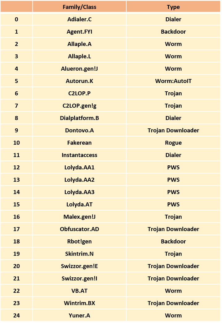
The Malimg Dataset contains 9339 malware images, belonging to 25 families/classes. Thus, Malware Detection can be achieved by performing a multi-class classification of malware.

The information regarding the dataset :

Dataset

Preprocessing

From binary to image

The Malimg dataset contains malware images which were converted from PE(Portable Executable) files to grey scale images. For each PE file, the raw data contains the hexadecimal representation of the file’s binary content. The goal is to convert those files into PNG images and use them as the input of our CNN.

To convert each malware file into grey scale image the following function can be used:

## This function allows us to process our hexadecimal files into png images##
def convertAndSave(array,name):
    print('Processing '+name)
    if array.shape[1]!=16: #If not hexadecimal
        assert(False)
    b=int((array.shape[0]*16)**(0.5))
    b=2**(int(log(b)/log(2))+1)
    a=int(array.shape[0]*16/b)
    array=array[:a*b//16,:]
    array=np.reshape(array,(a,b))
    im = Image.fromarray(np.uint8(array))
    im.save(root+'\\'+name+'.png', "PNG")
    return im

# Get the list of files
files=os.listdir(root)
print('files : ',files)
# We will process files one by one.
for counter, name in enumerate(files):
        #We only process .bytes files from our folder.
        if '.bytes' != name[-6:]:
            continue
        f=open(root+'/'+name)
        array=[]
        for line in f:
            xx=line.split()
            if len(xx)!=17:
                continue
            array.append([int(i,16) if i!='??' else 0 for i in xx[1:] ])
        plt.imshow(convertAndSave(np.array(array),name))
        del array
        f.close()

Here is the resulting image after converting the 0ACDbR5M3ZhBJajygTuf.bytes binary file into a PNG.

Grey Scale Image

Generating the dataset

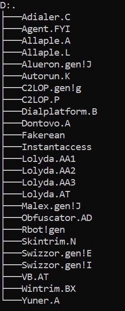
Here are our malware classes/families as subfolders containing PNGs:

Families

ImageDataGenerator.flow_from_directory() generates batches of normalized tensor image data from the respective data directories (families in our case). Thanks to this function, we can use our images for training and testing.

target_size: Resizes all images to the specified size. I chose (64*64) images.

batch_size: Is the size of the batch we will use. In our case, we only have 9339 images, thus setting a batch size above this value won’t change anything.

Once our batches have been generated, we can use the train_test_split() function to split data between train and test, following a (70–30) ratio. Here is the corresponding code :

from keras.preprocessing.image import ImageDataGenerator
from sklearn.model_selection import train_test_split

#Generating DataSet
path_root = "malimg_paper_dataset_imgs\\"
batches = ImageDataGenerator().flow_from_directory(directory=path_root, target_size=(64,64), batch_size=10000)
imgs, labels = next(batches)

#Split into train and test
X_train, X_test, y_train, y_test = train_test_split(imgs/255.,labels, test_size=0.3)

As you can see, the function well recognized the 25 classes thanks to the subfolders’ names.

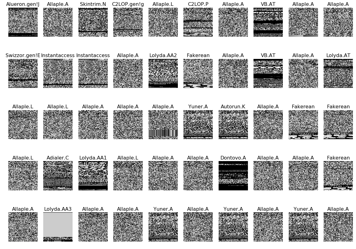
Here is a sample of our dataset :

FamiliyImages

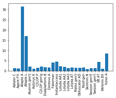
Quick Analysis

According to the following figure, More than 30% of images belong to class 2 : Allaple.A and 17% to class 3 : Allaple.L !

FamiliyPercentage

CNN model

Architecture

Now that our dataset is ready, we can build our model using Keras. The following structure will be used :

Convolutional Layer : 30 filters, (3 * 3) kernel size
Max Pooling Layer : (2 * 2) pool size
Convolutional Layer : 15 filters, (3 * 3) kernel size
Max Pooling Layer : (2 * 2) pool size
DropOut Layer : Dropping 25% of neurons.
Flatten Layer
Dense/Fully Connected Layer : 128 neurons, Relu activation function
DropOut Layer : Dropping 50% of neurons.
Dense/Fully Connected Layer : 50 neurons, Softmax activation function
Dense/Fully Connected Layer : num_class neurons, Softmax activation function

The input has a shape of [64 * 64 * 3] : [width * height * depth]. In our case, each Malware is a RGB image.

Here is the corresponding code :

def malware_model():
    Malware_model = Sequential()
    Malware_model.add(Conv2D(30, kernel_size=(3, 3),
                     activation='relu',
                     input_shape=(64,64,3)))
    Malware_model.add(MaxPooling2D(pool_size=(2, 2)))
    Malware_model.add(Conv2D(15, (3, 3), activation='relu'))
    Malware_model.add(MaxPooling2D(pool_size=(2, 2)))
    Malware_model.add(Dropout(0.25))
    Malware_model.add(Flatten())
    Malware_model.add(Dense(128, activation='relu'))
    Malware_model.add(Dropout(0.5))
    Malware_model.add(Dense(50, activation='relu'))
    Malware_model.add(Dense(num_classes, activation='softmax'))
    Malware_model.compile(loss='categorical_crossentropy', optimizer = 'adam', metrics=['accuracy'])
    return Malware_model

Unbalanced Data

Several methods are available to deal with unbalanced data. To give higher weight to minority class and lower weight to the majority class, sklearn.utilis.class_weights function uses the values of y to automatically adjust weights inversely proportional to class frequencies in the input data. To use this method, y_train must not be one-hot encoded.

from sklearn.utils import class_weight

y_train_new = np.argmax(y_train, axis=1)
#Deal with unbalanced Data
class_weights = class_weight.compute_class_weight('balanced',
                                                 np.unique(y_train_new),
                                                 y_train_new)
 #Train and test our model                        
Malware_model.fit(X_train, y_train, validation_data=(X_test, y_test), epochs=10,  class_weight=class_weights)
scores = Malware_model.evaluate(X_test, y_test)

                                           . . .

Results

After training and testing our model, we reach a final accuracy of 95%.

Accuracy

Plotting the confusion matrix can give us graphical representaion of our classification.

ConfusionMatrix

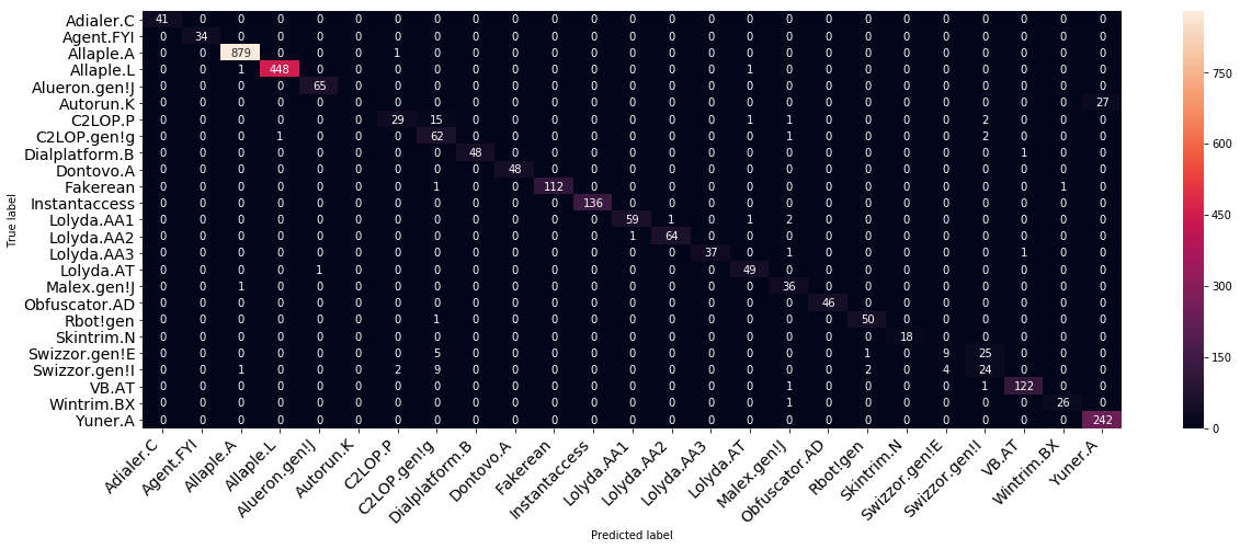
We can observe that although most of the Malwares were well classified, Autorun.K is always mistaken for Yuner.A. This is probably because we have very few samples of Autorun.K in our dataset and that both are part of a close Worm type.

Moreover, Swizzor.gen!E is often mistaken with Swizzor.gen!l, which can be explained by the fact that they come from really close kind of families and types and thus could have similarities in their code.

Conclusion

That’s it! With this you can now be able to build your malware images dataset and use it to perform multi-class classification for detection thanks to Convolutional Neural Networks.

MalwareDetection

Malware Detection using Deep Learning

Detailed Explaination for Malware Detection Using Deep Learning:

Dataset

Preprocessing

From binary to image

Generating the dataset

Quick Analysis

CNN model

Architecture

Unbalanced Data

Results

Conclusion